Extensive scaling tests on the new trackerless Streamr Network 1.0 were run in early 2025 to confirm that the new architecture met expectations for performance and scalability. Thousands of nodes were deployed across 17 regions worldwide, using data centers to simulate a global live network.
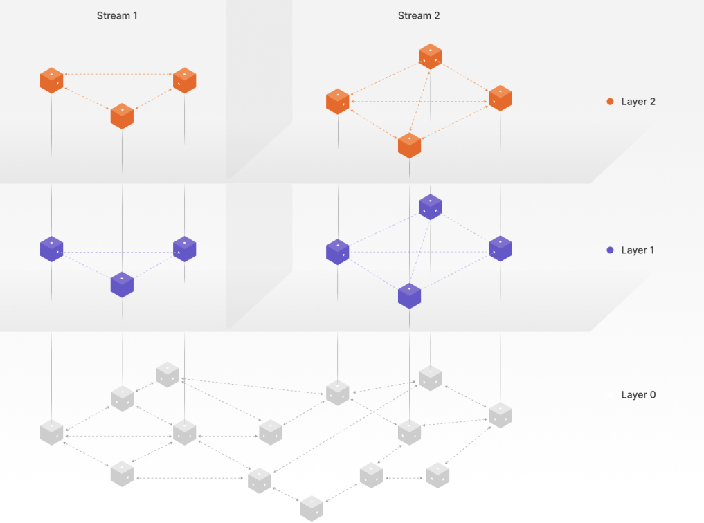
In Part 1, we explored the three-layer trackerless architecture that replaced the old tracker model. In this follow-up, Part 2, we put that design to the test — validating locality awareness in Layer 2 and measuring how the network performs at scale.
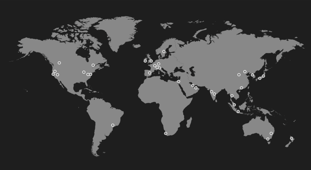
17 regions in AWS were configured to run EC2 instances which contain Streamr Network nodes.
Table of Contents
Experiment Setup
Most experiments were run with up to ~2,000 nodes. A centralized script coordinated the experiments, tracking progress and sending instructions to the nodes.
As a baseline, pings were sent between AWS regions to measure latencies. This gave a ground truth for expected operation times. The measured mean one-way delay between the regions was 75 ms.
Metrics Analyzed
The tests measured:
- Join time: Time for a node to join the Layer 0 DHT.
- Routing time: Average time to route a message from each node to each node.
- Stream message propagation delay: Time for each node in a stream to receive a message (CDF).
- Time to data: Time for a node to begin receiving data after starting, including fetching entry point data and joining Layer 1.
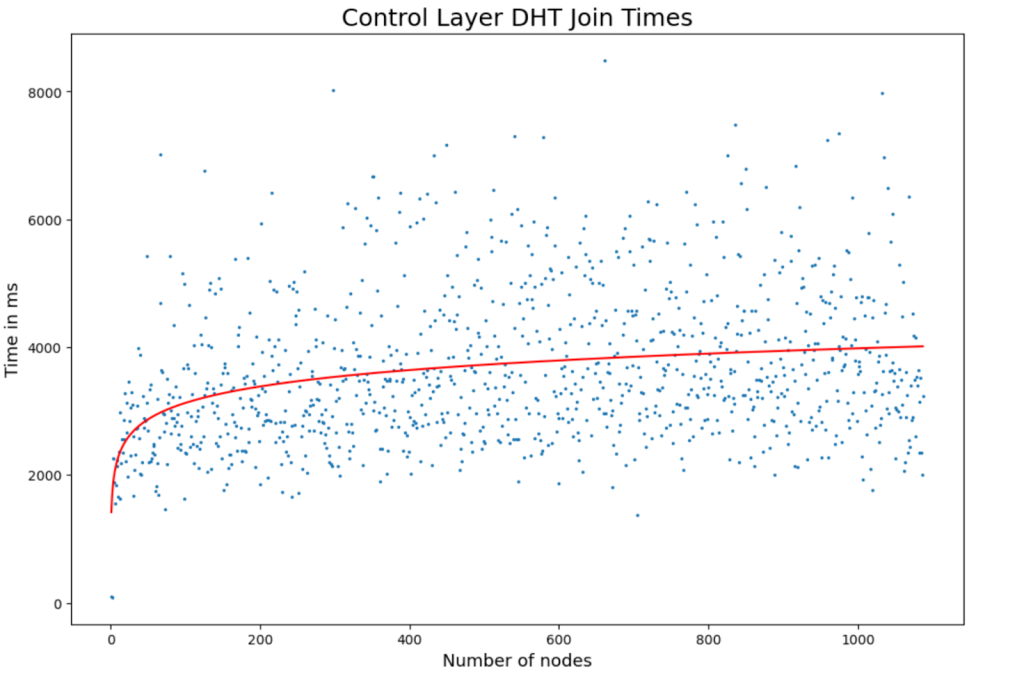
Measuring Layer 0 DHT Join Times
Nodes were instructed to join the Layer 0 DHT one by one. This simplest experiment showed a logarithmic curve for join times. Some variance was observed, with nodes taking up to 8 seconds to fully join the DHT.
This is not problematic because nodes can begin participating in higher layers once a single DHT connection is established — they don’t need to wait for full DHT sync.
Measuring Layer 0 Routing Delays and Hops
The next experiment measured routing delays and hops in the DHT. Multiple runs were performed with increasing numbers of nodes, scaling up to more than 2,000 nodes in total.
Each node first joined the Layer 0 DHT, then routed requests to every other node. From this we calculated the mean number of hops and the mean RTT (round-trip time) for routed requests.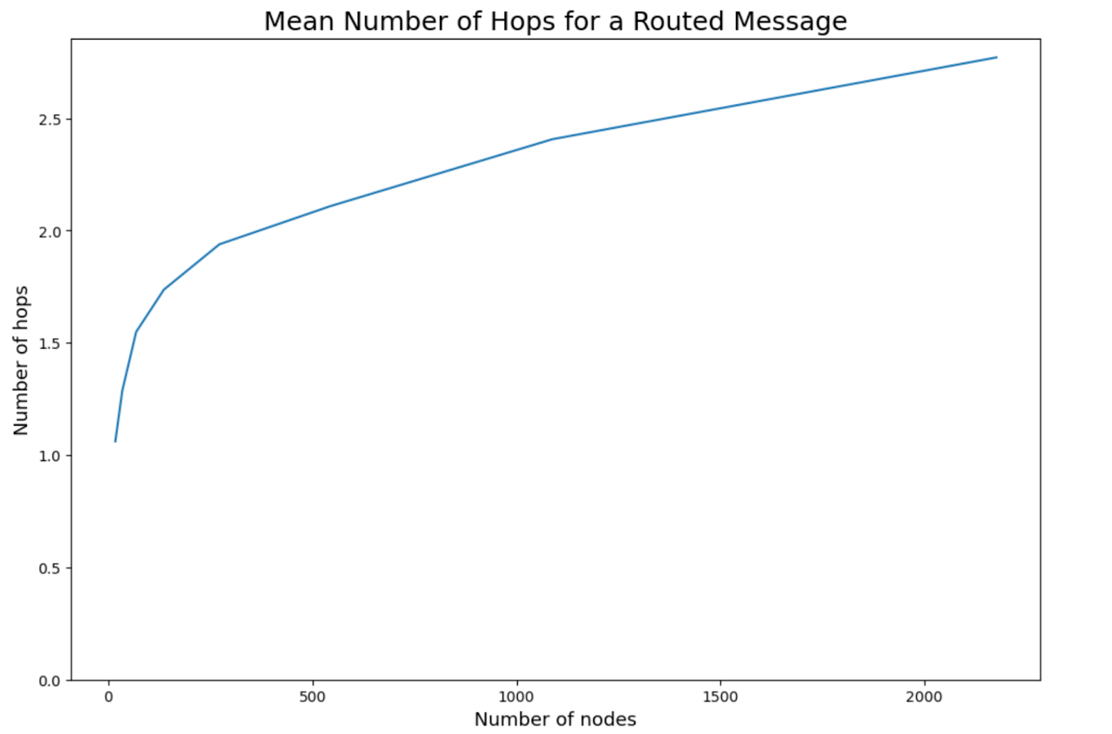
The mean hop count grew logarithmically as the number of nodes increased. At 2,000 nodes, routing a message required fewer than 3 hops on average.
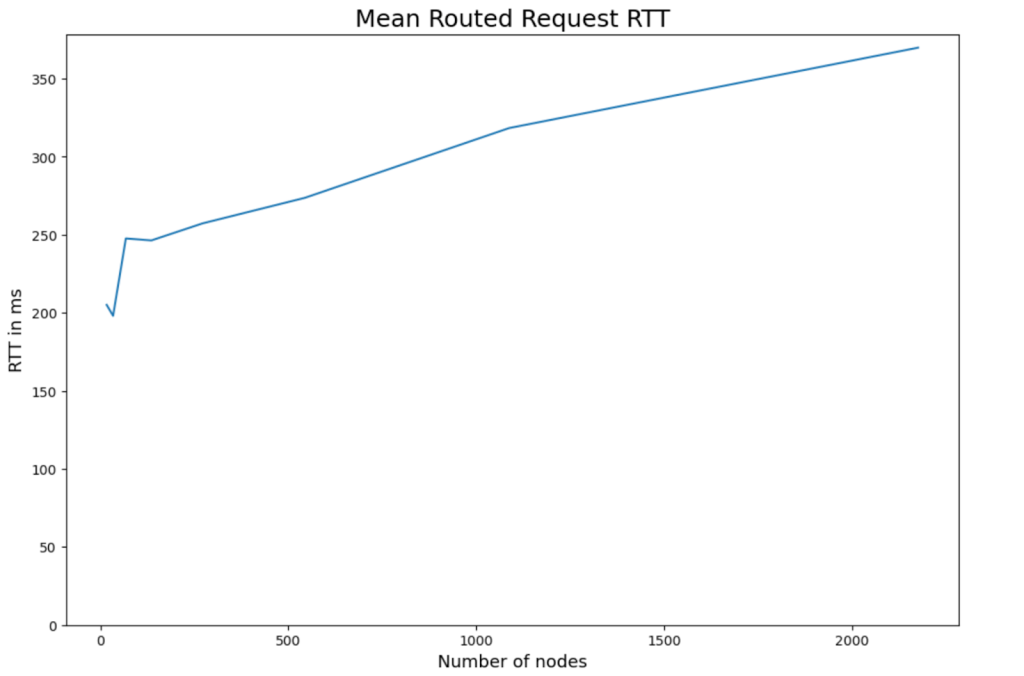
Mean RTTs also grew logarithmically, although the curve was less smooth than hop counts. This is due to how AWS distributes IP addresses: DHT IDs derive their most significant bits from the node’s IP address. Because AWS allocates addresses in clusters, the distribution was less uniform than randomly selected DHT IDs would have been.
As a result, RTT performance in the experiment was slightly worse than the theoretical optimum. Even so, at 2,000 nodes the average RTT for routing a request and response was still around 360 ms.
This result is crucial: efficient Layer 0 routing underpins the higher layers of the Streamr Network. Layer 1, for example, relies heavily on Layer 0 routing for signaling, and all WebSocket/WebRTC connection establishment also depends on it.
Measuring Stream Message Propagation Delays
To measure stream message propagation we started an increasing number of nodes similarly to the routing test up to 2000 nodes. In the beginning the nodes were started and were instructed to join a given stream partition. Once all nodes had successfully joined, we published a message from each node to the stream. All nodes would store the time it took for them to receive the message. This allowed us to calculate the mean message propagation delays and relative delay penalties in layer2. In the following graphs, the thick line represents the mean value of repeated experiment runs and the highlighted area represents the min and max mean value of the repeats.
The mean message propagation delay is higher for smaller streams than it is for larger streams. This is the expected behaviour as in larger streams the location aware clustering takes stronger effect. We see the mean message propagation delays flatline after 2000 nodes in the experiments.
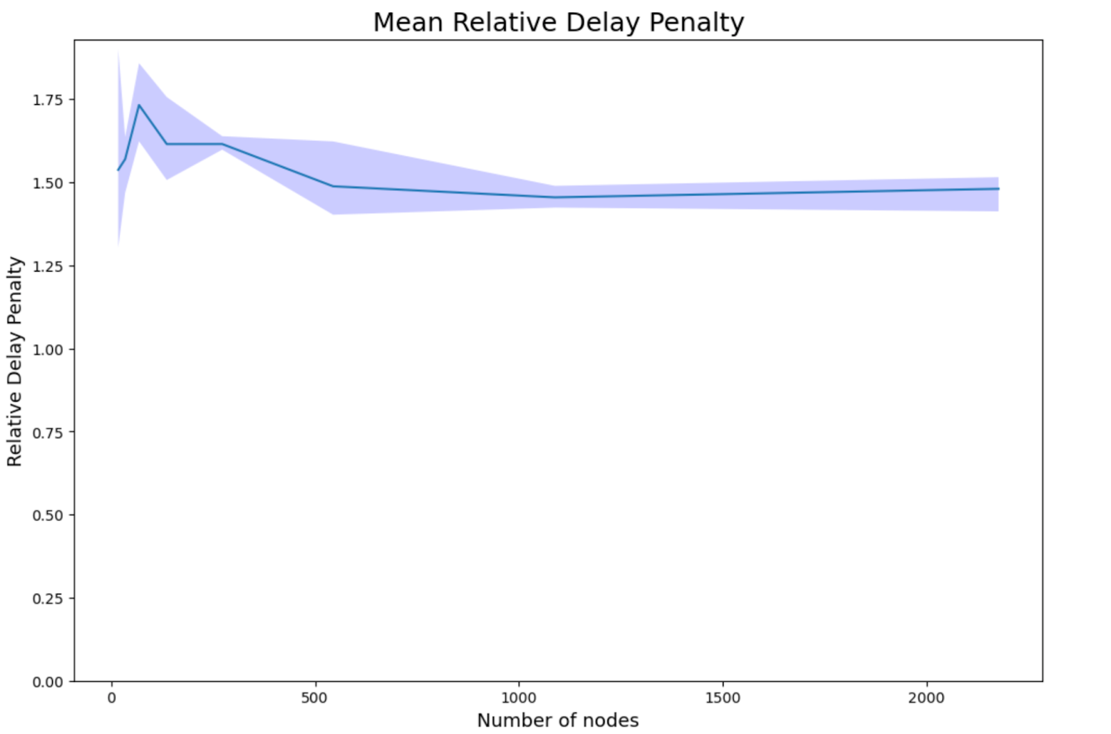
For relative delay penalties we took the mean message propagation delays and the mean of the underlying latencies in the experiments. This metric is used to estimate the latency cost of sending a message over the layer2 network when compared to sending the message over a direct wire. From the results we can see that the relative delay penalties are quite low. 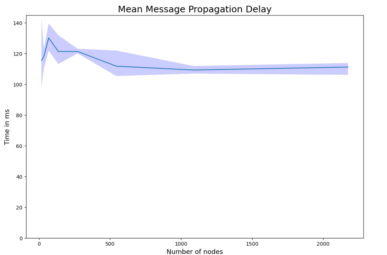
Time to Data Measurements
To measure time to data, more than 2,000 nodes were started one by one and instructed to join a given stream partition. Before the subscribing nodes came online, a publishing node was added to the network. This publisher sent data to the stream at a fixed interval of 200 ms.
Each subscribing node recorded:
- The time to fetch stream entry point data from the Layer 0 DHT.
- The Layer 1 DHT join time.
- The time to open the first neighbor connection in the stream.
- The time to receive its first content data point.

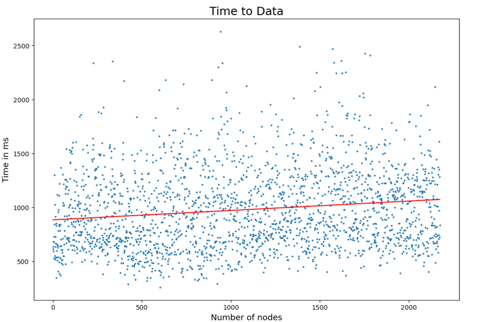
The goal was for the mean time to data to remain below 2 seconds. In practice, the mean was consistently around 1 second across all network sizes — a very positive result.
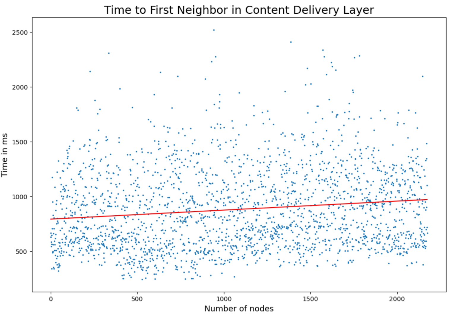
We also measured time to first neighbor, which indicates how quickly a node establishes its first Layer 2 connection. Once that connection is open, the node is ready to broadcast or receive data.
During these tests, we also measured the average time to run DHT queries, since these are crucial for finding entry point nodes for stream partitions. On average, DHT queries took ~216 ms at all network sizes.
The time to first neighbor metric combines:
- The DHT query
- Routing a request to the stream entry points
- Establishing the first neighbor connection
From the results:
- Mean time to data: ~820 ms
- Mean time to first neighbor: ~720 ms
Experiment Recap
By incrementally scaling the number of nodes and measuring multiple performance metrics, we observed the following:
- Join times remained short: Nodes became functional quickly without waiting for full DHT sync. As soon as a single connection was established, nodes could start receiving data.
- Fast peer discovery: Time to first neighbor was very low, allowing nodes to begin relaying or receiving data almost immediately. Mean time to data averaged around 1 second, with only a few outliers taking longer.
- Minimal increase in hop counts: Routing efficiency scaled as expected. Even with thousands of nodes, the average number of hops grew only logarithmically. Doubling the network size did not significantly increase hops. This is exactly what Kademlia DHT predicts — and the experiments confirmed it.
- Sub-linear latency growth: Latency metrics increased slower than the growth in network size. In fact, larger networks benefited from location-aware clustering, which reduced propagation delays.
- Stable performance curves: No sudden degradation or tipping points were observed. Metrics followed smooth logarithmic curves, suggesting the network could scale to even larger node counts without surprises.
- Balanced bandwidth usage: Although not detailed in graphs, bandwidth distribution was implied. Each node only forwards data for streams it subscribes to. In well-subscribed streams, the relay load is shared — as more subscribers join, the work is collectively balanced.
- Low relative path delay: Measured at ~1.6× compared to a direct wire across all network sizes. With only ~4 connections per node, this is an excellent result.
Conclusion
The new trackerless Streamr Network performs as well as, or better than, the old tracker-based model it replaced.
- It consistently met the <2s target for data availability.
- Latency increased sub-linearly with network size. For example, scaling from 500 to 2,000 nodes added only tens of milliseconds to the average propagation time.
- Routing scaled logarithmically: doubling the number of nodes did not significantly increase hop counts.
- The combination of layered architecture and locality awareness ensures smooth performance at scale.
In other words: the trackerless design has proven itself — not just in theory, but under large-scale, global test conditions.
If you have any questions about the blog, feel free to ask on the Streamr Discord.