The Corea milestone of the Streamr Network went live in late 2019. Since then a few people in the team have been working on an academic whitepaper to describe its design principles, position it with respect to prior art, and prove certain properties it has. The paper is now ready, and it has been submitted to the IEEE Access journal for peer review. It is also now published on the new Papers section on the project website. In this blog, I’ll introduce the paper and explain its key results. All the figures presented in this post are from the paper.
The reasons for doing this research and writing this paper were simple: many prospective users of the Network, especially more serious ones such as enterprises, ask questions like how does it scale, why does it scale, what is the latency in the network, and how much bandwidth is consumed? While some answers could be provided before, the Network in its currently deployed form is still small-scale and can’t really show a track record of scalability for example, so there was clearly a need to produce some in-depth material about the structure of the Network and its performance on a large, global scale. The paper answers these questions.
Another reason is that decentralized peer-to-peer networks have experienced a new renaissance due to the rise in blockchain networks. Peer-to-peer pub/sub networks were a hot research topic in the early 2000s, but not many real-world implementations were ever created. Today, most blockchain networks use methods from that era under the hood to disseminate block headers, transactions, and other events important for them to function. Other megatrends like IoT and social media are also creating demand for new kinds of scalable message transport layers.
Table of Contents
The latency vs. bandwidth tradeoff
The current Streamr Network uses regular random graphs as stream topologies. ‘Regular’ here means that nodes connect to a fixed number of other nodes that publish or subscribe to the same stream, and ‘random’ means that those nodes are selected randomly.
Random connections can of course mean that absurd routes get formed occasionally, for example a data point might travel from Germany to France via the US. But random graphs have been studied extensively in the academic literature, and their properties are not nearly as bad as the above example sounds – such graphs are actually quite good! Data always takes multiple routes in the network, and only the fastest route counts. The less-than-optimal routes are there for redundancy, and redundancy is good, because it improves security and churn tolerance.
There is an important parameter called node degree, which is the fixed number of nodes to which each node in a topology connects. A higher node degree means more duplication and thus more bandwidth consumption for each node, but it also means that fast routes are more likely to form. It’s a tradeoff; better latency can be traded for worse bandwidth consumption. In the following section, we’ll go deeper into analyzing this relationship.
Network diameter scales logarithmically
One useful metric to estimate the behavior of latency is the network diameter, which is the number of hops on the shortest path between the most distant pair of nodes in the network (i.e. the “longest shortest path”. The below plot shows how the network diameter behaves depending on node degree and number of nodes.
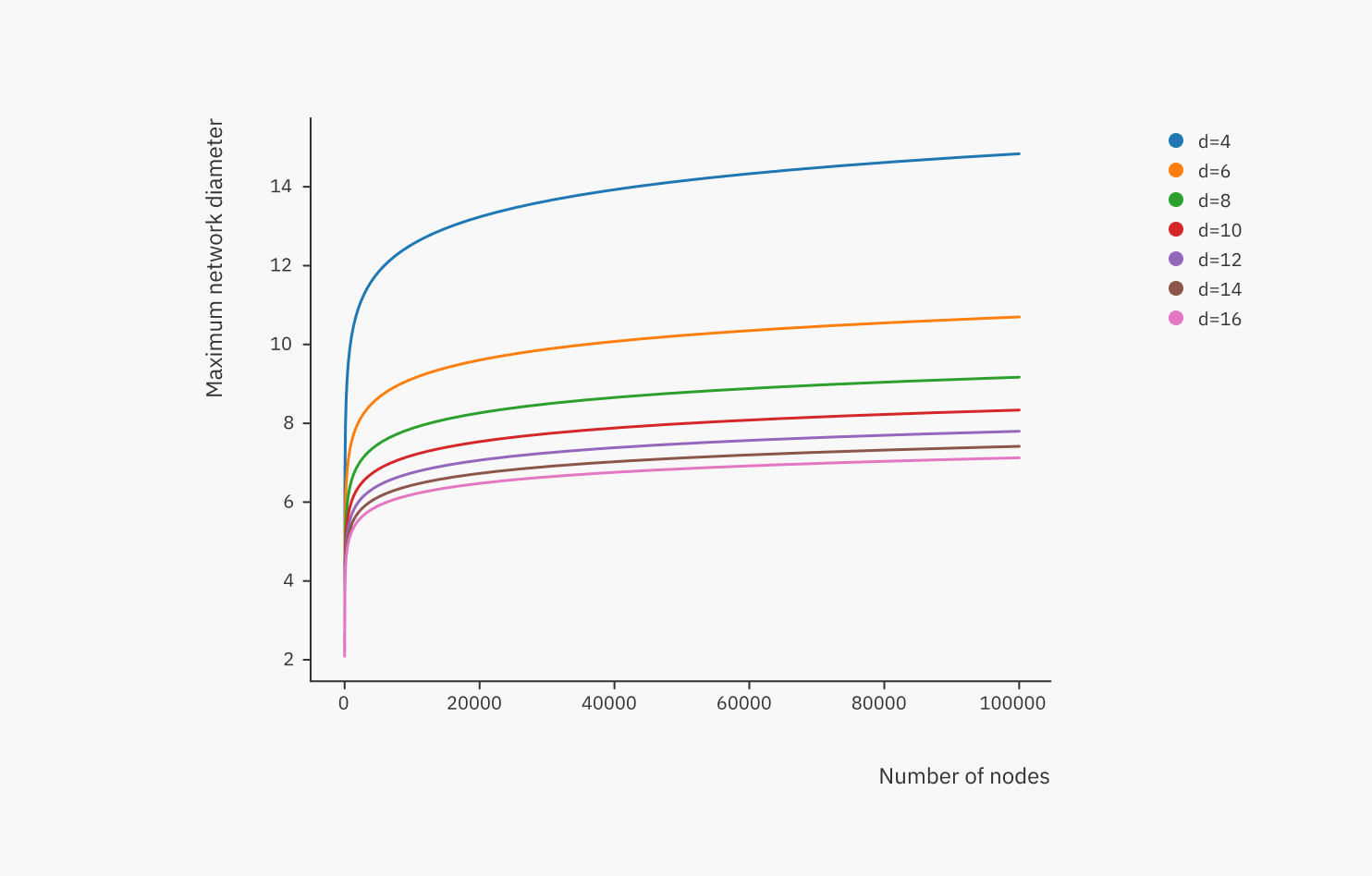
We can see that the network diameter increases logarithmically (very slowly), and a higher node degree ‘flattens the curve’. This is a property of random regular graphs, and this is very good – growing from 10,000 nodes to 100,000 nodes only increases the diameter by a few hops! To analyze the effect of the node degree further, we can plot the maximum network diameter using various node degrees:
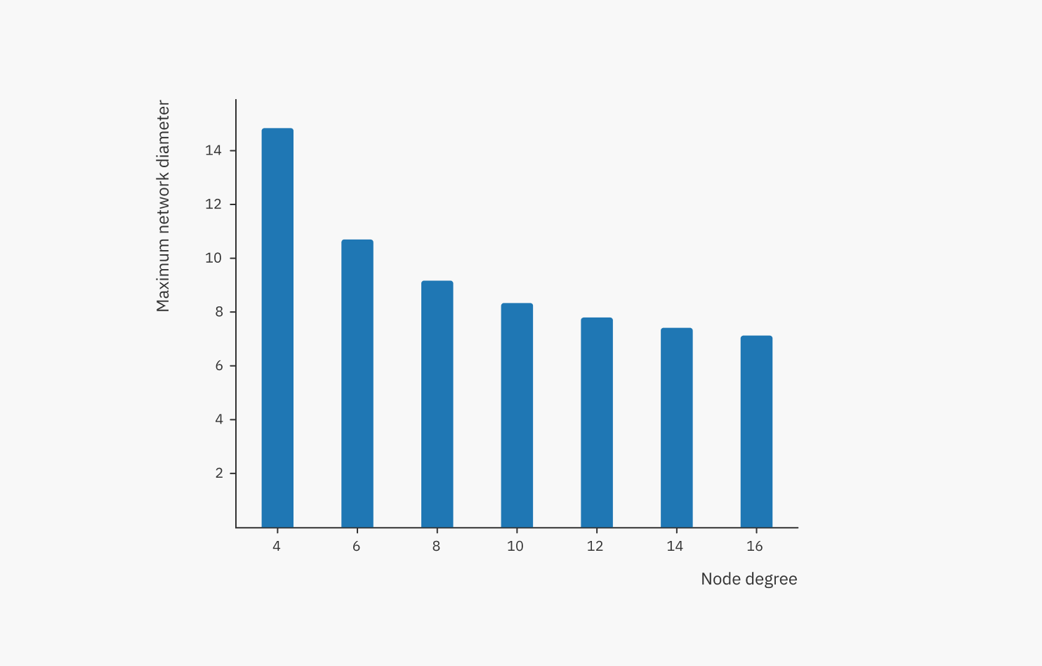
We can see that there are diminishing returns for increasing the node degree. On the other hand, the penalty (number of duplicates, i.e. bandwidth consumption), increases linearly with node degree:
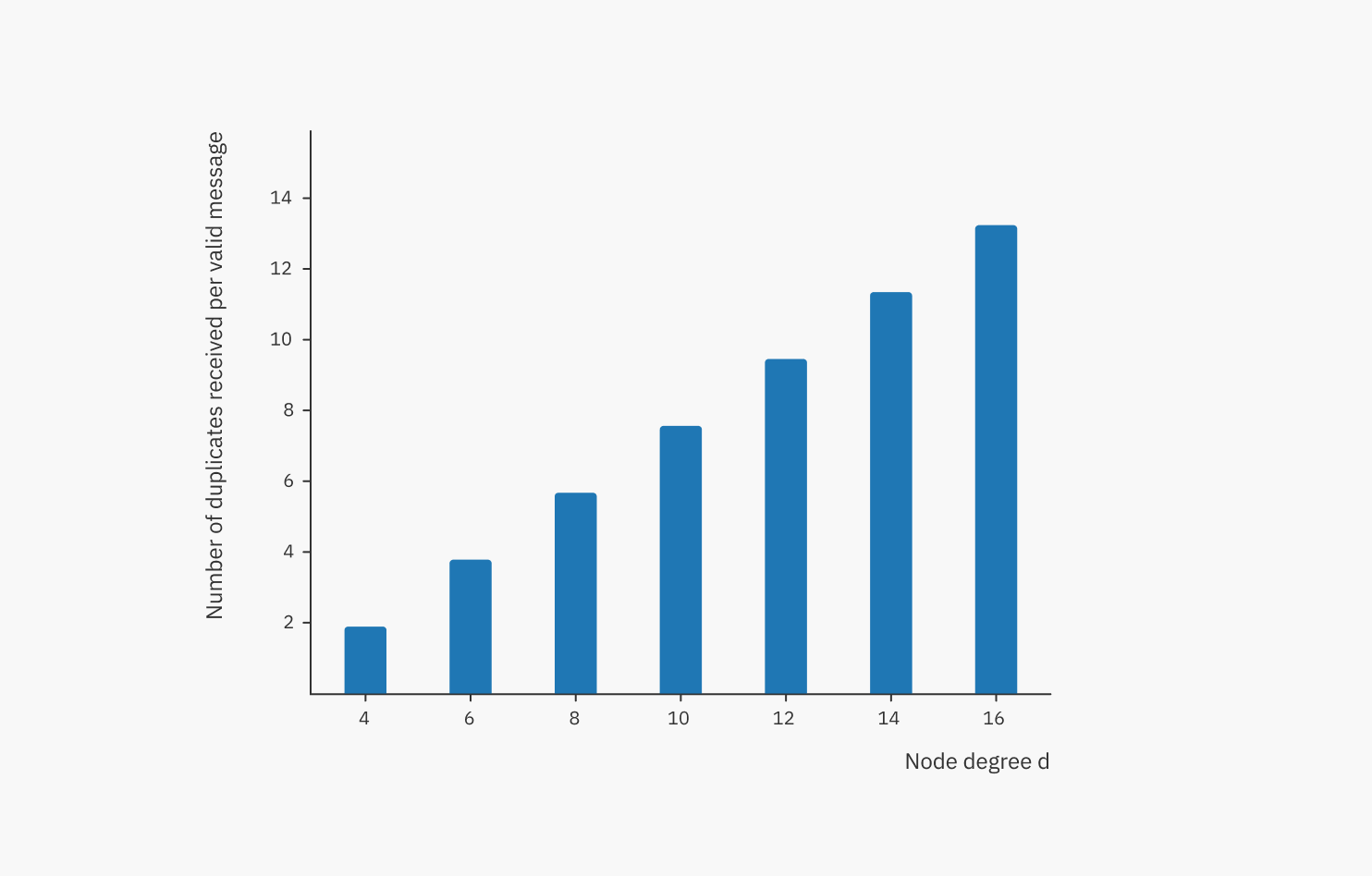
In the Streamr Network, each stream forms its own separate overlay network and can even have a custom node degree. This allows the owner of the stream to configure their preferred latency/bandwidth balance (imagine such a slider control in the Streamr Core UI). However, finding a good default value is important. From this analysis, we can conclude that:
- The logarithmic behavior of network diameter leads us to hope that latency might behave logarithmically too, but since the number of hops is not the same as latency (in milliseconds), the scalability needs to be confirmed in the real world (see next section).
- A node degree of 4 yields good latency/bandwidth balance, and we have selected this as the default value in the Streamr Network. This value is also used in all the real-world experiments described in the next section.
It’s worth noting that in such a network, the bandwidth requirement for publishers is determined by the node degree and not the number of subscribers. With a node degree of 4 and a million subscribers, the publisher only uploads 4 copies of a data point, and the million subscribing nodes share the work of distributing the message among themselves. In contrast, a centralized data broker would need to push out a million copies.
Latency scales logarithmically
To see if actual latency scales logarithmically in real-world conditions, we ran large numbers of nodes in 16 different Amazon AWS data centers around the world. We ran experiments with network sizes between 32 to 2048 nodes. Each node published messages to the network, and we measured how long it took for the other nodes to get the message. The experiment was repeated 10 times for each network size.
The below image displays one of the key results of the paper. It shows a CDF (cumulative distribution function) of the measured latencies across all experiments. The y-axis runs from 0 to 1, i.e. 0% to 100%.
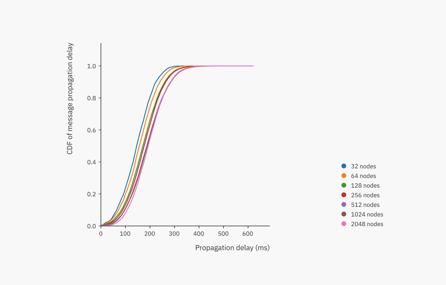
From this graph we can easily read things like: in a 32 nodes network (blue line), 50% of message deliveries happened within 150 ms globally, and all messages were delivered in around 250 ms. In the largest network of 2048 nodes (pink line), 99% of deliveries happened within 362 ms globally.
To put these results in context, PubNub, a centralized message brokering service, promises to deliver messages within 250 ms – and that’s a centralized service! Decentralization comes with unquestionable benefits (no vendor lock-in, no trust required, network effects, etc.), but if such protocols are inferior in terms of performance or cost, they won’t get adopted. It’s pretty safe to say that the Streamr Network is on par with centralized services even when it comes to latency, which is usually the Achilles’ heel of P2P networks (think of how slow blockchains are!). And the Network will only get better with time.
Then we tackled the big question: does the latency behave logarithmically?
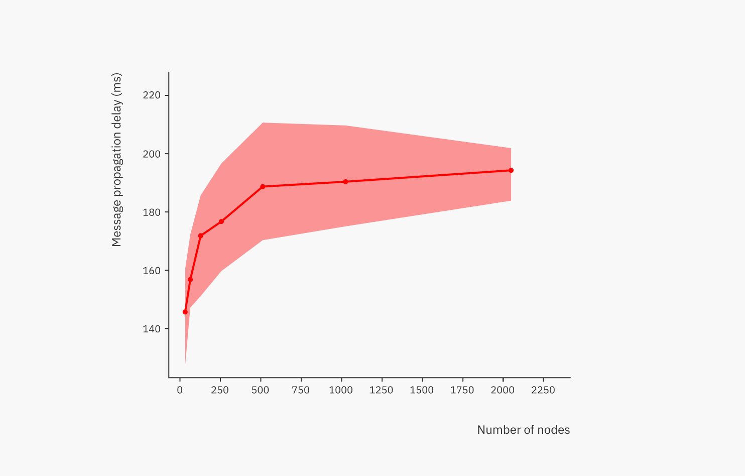
Above, the thick line is the average latency for each network size. From the graph, we can see that the latency grows logarithmically as the network size increases, which means excellent scalability.
The shaded area shows the difference between the best and worst average latencies in each repeat. Here we can see the element of chance at play; due to the randomness in which nodes become neighbours, some topologies are faster than others. Given enough repeats, some near-optimal topologies can be found. The difference between average topologies and the best topologies gives us a glimpse of how much room for optimization there is, i.e. with a smarter-than-random topology construction, how much improvement is possible (while still staying in the realm of regular graphs)? Out of the observed topologies, the difference between the average and the best observed topology is between 5-13%, so not that much. Other subclasses of graphs, such as irregular graphs, trees, and so on, can of course unlock more room for improvement, but they are different beasts and come with their own disadvantages too.
It’s also worth asking: how much worse is the measured latency compared to the fastest possible latency, i.e. that of a direct connection? While having direct connections between a publisher and subscribers is definitely not scalable, secure, or often even feasible due to firewalls, NATs and such, it’s still worth asking what the latency penalty of peer-to-peer is.
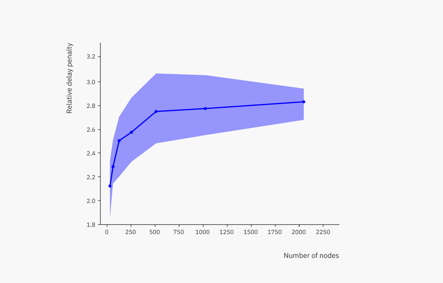
As you can see, this plot has the same shape as the previous one, but the y-axis is different. Here, we are showing the relative delay penalty (RDP). It’s the latency in the peer-to-peer network (shown in the previous plot), divided by the latency of a direct connection measured with the ping tool. So a direct connection equals an RDP value of 1, and the measured RDP in the peer-to-peer network is roughly between 2 and 3 in the observed topologies. It increases logarithmically with network size, just like absolute latency.
Again, given that latency is the Achilles’ heel of decentralized systems, that’s not bad at all. It shows that such a network delivers acceptable performance for the vast majority of use cases, only excluding the most latency-sensitive ones, such as online gaming or arbitrage trading. For most other use cases, it doesn’t matter whether it takes 25 or 75 milliseconds to deliver a data point.
Latency is predictable
It’s useful for a messaging system to have consistent and predictable latency. Imagine for example a smart traffic system, where cars can alert each other about dangers on the road. It would be pretty bad if, even minutes after publishing it, some cars still haven’t received the warning. However, such delays easily occur in peer-to-peer networks. Everyone in the crypto space has seen first-hand how plenty of Bitcoin or Ethereum nodes lag even minutes behind the latest chain state.
So we wanted to see whether it would be possible to estimate the latencies in the peer-to-peer network if the topology and the latencies between connected pairs of nodes are known. We applied Dijkstra’s algorithm to compute estimates for average latencies from the input topology data, and compared the estimates to the actual measured average latencies:
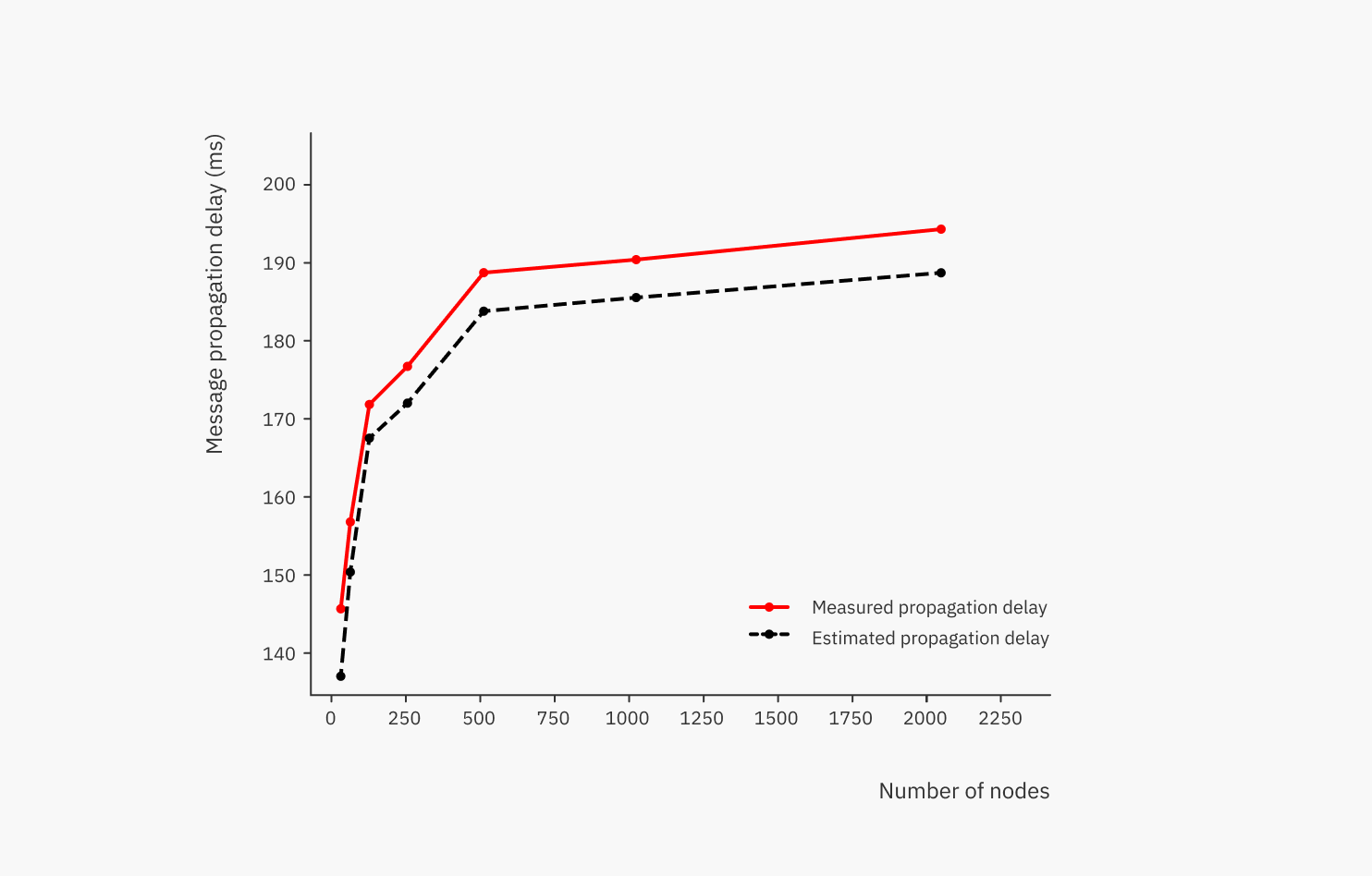
We can see that, at least in these experiments, the estimates seemed to provide a lower bound for the actual values, and the average estimation error was 3.5%. The measured value is higher than the estimated one because the estimation only considers network delays, while in reality there is also a little bit of a processing delay at each node.
Conclusion
The research has shown that the Streamr Network can be expected to deliver messages in roughly 150-350 milliseconds worldwide, even at a large scale with thousands of nodes subscribing to a stream. This is on par with centralized message brokers today, showing that the decentralized and peer-to-peer approach is a viable alternative for all but the most latency-sensitive applications.
It’s thrilling to think that by accepting a latency only 2-3 times longer than the latency of an unscalable and insecure direct connection, applications can interconnect over an open fabric with global scalability, no single point of failure, no vendor lock-in, and no need to trust anyone – all that becomes available out of the box.
In the real-time data space, there are plenty of other aspects to explore, which we didn’t cover in this paper. For example, we did not measure throughput characteristics of network topologies. Different streams are independent, so clearly there’s scalability in the number of streams, and heavy streams can be partitioned, allowing each stream to scale too. Throughput is mainly limited, therefore, by the hardware and network connection used by the network nodes involved in a topology. Measuring the maximum throughput would basically be measuring the hardware, as well as the performance, of our implemented code. While interesting, this is not a high priority research target at this point in time. And thanks to the redundancy in the network, individual slow nodes do not slow down the whole topology; the data will arrive via faster nodes instead.
Also out of scope for this paper is analyzing the costs of running such a network, including the OPEX for publishers and node operators. This is a topic of ongoing research, which we’re currently doing as part of designing the token incentive mechanisms of the Streamr Network, due to be implemented in a later milestone.
I hope that this blog has provided some insight into the fascinating results the team uncovered during this research. For a more in-depth look at the context of this work, and more detail about the research, we invite you to read the full paper.
If you have an interest in network performance and scalability from a developer or enterprise perspective, we will be hosting a talk about this research in the coming weeks, so keep an eye out for more details on the Streamr social media channels. In the meantime, feedback and comments are welcome. Please add a comment to this Reddit thread or email contact@streamr.network.